Blog
Where Is Recursive Self-Improvement Possible?
Sustained recursive self-improvement depends on the process that generates tasks as well as on the learner. It requires tasks in which each learned abstraction makes the next one cheaper to discover.
What Would Count as Recursive Self-Improvement? separated improvements to an object, such as a tool, a prompt, a cached solution, or a tuned learning rate, from improvements to the mechanism that produces later improvements. An improved object can raise performance while leaving the next discovery as hard as before. The recursive part is isolated by comparing the improved system with a frozen-mechanism counterfactual that inherits the same installed gains and keeps the old improvement process.
The comparison detects recursive improvement once it occurs and leaves open where to expect it. A current form of the question is whether AI progress will stay concentrated in mathematics and code, where reinforcement learning can use exact verifiers, while less verifiable domains level off because they keep depending on new information produced by people.
An ideal learner extracts every usable regularity from the data it receives, and it can still exploit only the structure that the task-generating process contains. The capability of an ideal learner can therefore level off, and recursive self-improvement (RSI) is a joint property of the learner and the task-generating process.
The property required of the task-generating process is stronger than predictability, compositionality, or unbounded complexity. Sustained RSI requires recursive abstraction structure, in which abstractions learned earlier become tools that make later abstractions cheaper to discover. Different amounts of this structure lead to different scaling regimes for the same ideal learner.
Benchmark curves and capability curves
Language-model loss, minus an irreducible term, has followed approximate power laws in training compute over many orders of magnitude (Kaplan et al., 2020; Hoffmann et al., 2022),
\[\epsilon(C) \approx A\, C^{-\alpha} ,\]
where \(C\) is training compute and \(\epsilon\) is the reducible part of the loss. Taking \(\theta = -\log \epsilon\) as a latent capability coordinate gives
\[\theta(C) = a + b \log C ,\]
with \(a = -\log A\) and \(b = \alpha\), so multiplying compute by a constant factor adds a constant amount of latent capability.
Benchmark scores can follow a different curve. In item response theory, the probability that a model with ability \(\theta\) solves item \(i\) depends on the difference between \(\theta\) and the difficulty \(d_i\) of the item,
\[P_i(\text{success} \mid \theta) = \sigma\bigl(\kappa_i(\theta - d_i)\bigr) ,\]
where \(\sigma\) is the logistic function and the discrimination \(\kappa_i\) sets how fast the success probability rises as \(\theta\) passes \(d_i\). Truong et al. (2026) estimate scaling laws with this factorization into model ability and item difficulty. Averaged over a distribution \(\mu\) of tasks, the benchmark score is
\[S_\mu(C) = \mathbb E_{i \sim \mu}\Bigl[\sigma\bigl(\kappa_i(\theta(C) - d_i)\bigr)\Bigr] .\]
In the limit \(\kappa_i \to \infty\), each success probability becomes a step function \(\mathbf 1[\theta \ge d_i]\), and
\[S_\mu(C) = F_\mu\bigl(a + b \log C\bigr) ,\]
where \(F_\mu\) is the cumulative distribution function of task difficulty under \(\mu\). The relation holds for any distribution of difficulty, so the same learner can produce very different benchmark curves. If difficulties are spread evenly over \(\theta\), the score rises roughly linearly in \(\log C\). If they cluster around one value, the score stays flat and then jumps. A gap in the distribution produces a plateau, and a distribution with several modes produces several apparent emergences.

Differentiating the score gives
\[\frac{dS_\mu}{d\log C} = f_\mu(\theta)\, \frac{d\theta}{d\log C} ,\]
where \(f_\mu\) is the density of task difficulty. The slope of a benchmark curve is the product of how many tasks lie at the current ability level and how fast the learner gains ability per unit of log compute. A sudden jump in a benchmark score is therefore consistent with smooth change inside the model. Schaeffer et al. (2023) showed that nonlinear metrics can produce apparent emergence from smooth underlying improvement, and a concentrated distribution of difficulty has the same effect. The shape of a benchmark curve mixes the distribution of task difficulty with the dynamics of learning, and the two have to be separated before the curve can serve as evidence for RSI.
Learning efficiency as a function of capability
With \(\tau = \log C\), ordinary scaling has a constant slope, \(d\theta/d\tau = b\), so each unit of log compute buys the same amount of latent capability. If accumulated capability changes how efficiently later capability is gained, the slope becomes a function of capability,
\[\frac{d\theta}{d\tau} = \beta(\theta) ,\]
and the scaling law depends on the state of the learner. Inverting the equation gives the compute needed to go from \(\theta_0\) to a target \(\Theta\),
\[\log \frac{C(\Theta)}{C_0} = \int_{\theta_0}^{\Theta} \frac{du}{\beta(u)} .\]
With constant efficiency \(\beta = b\), the required compute \(C(\Theta) = C_0\, e^{(\Theta - \theta_0)/b}\) grows exponentially with the target, so linear gains in capability cost exponentially more compute. With efficiency that rises linearly with capability, \(\beta(\theta) = b + k\theta\), the solution grows as \(\theta \propto C^{k}\) for large \(C\). Capability then grows polynomially in compute, and the scaling law itself has changed.
Advantage over a frozen mechanism
Let \(\beta_F(\theta)\) be the learning efficiency of the frozen-mechanism counterfactual, and \(\beta_R(\theta)\) the efficiency of the system that keeps its recursive improvements. If both start from the same capability with the same compute, the logarithm of the ratio of their compute requirements at a target \(\Theta\) is
\[\log \frac{C_F(\Theta)}{C_R(\Theta)} = \int_{\theta_0}^{\Theta} \Bigl(\frac{1}{\beta_F} - \frac{1}{\beta_R}\Bigr)\, d\theta .\]
The recursive system has an unbounded compute advantage, \(C_R(\Theta) = o\bigl(C_F(\Theta)\bigr)\), when the integral diverges as \(\Theta \to \infty\). Small advantages can add up to an unbounded total, so the condition can hold even when every individual recursive improvement is small.
The discrete version of the condition is a product of per-step factors. If improvement \(n\) makes the next discovery cheaper by a factor \(\rho_n\), the cumulative advantage after \(N\) improvements is \(\prod_{n=1}^{N} \rho_n\), which is unbounded when the sum \(\sum_n \log \rho_n\) diverges. With \(\rho_n = 1 + 1/n\), the product equals \(N + 1\), which is unbounded even though \(\rho_n \to 1\). With \(\rho_n = 1 + 1/n^2\), every step is still an improvement, but the product converges to about 3.68. Improvement at every step is therefore a weaker property than an unbounded cumulative advantage.
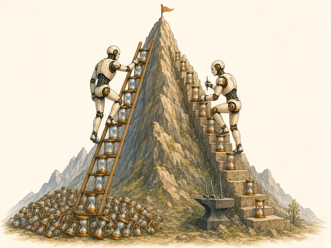
Frontier difficulty and reusable leverage
The efficiency can be split into two factors,
\[\frac{1}{\beta(\theta)} = \frac{H(\theta)}{R(\theta)} ,\]
where \(H(\theta)\) is the intrinsic difficulty of the next capability frontier and \(R(\theta)\) is the reusable leverage supplied by everything learned so far. A single scaling curve identifies only their ratio. A frozen and a recursive system at the same capability face the same frontier, however, so the ratio of their efficiencies, \(\beta_R/\beta_F = R_R/R_F\), depends only on their reusable leverage.
Taking logarithmic derivatives gives
\[\frac{d \log \beta}{d\theta} = r(\theta) - h(\theta) ,\]
where \(r = d \log R/d\theta\) is the growth rate of reusable leverage and \(h = d \log H/d\theta\) is the growth rate of frontier difficulty. The sign of \(r - h\) defines three regimes. When \(r < h\), frontier difficulty grows faster than reusable leverage, efficiency falls, and returns to log compute diminish, with capability saturating if efficiency reaches zero at a finite level. When \(r = h\), reuse offsets the growth in difficulty, efficiency stays constant, and capability grows linearly in log compute, as in ordinary scaling. When \(r > h\), reusable leverage grows faster than frontier difficulty, efficiency rises, and capability accelerates relative to log compute.
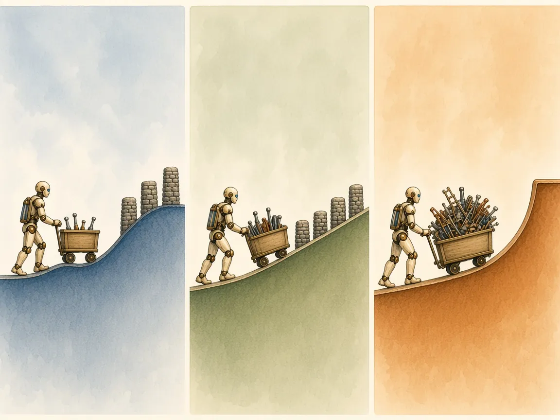
Recursive acceleration requires the third regime. Whether a learner can stay in it depends on the task-generating process as well as on the learner, because the amount and organization of reusable structure in the tasks limit how fast \(R\) can grow.
Transfer and recursive abstraction
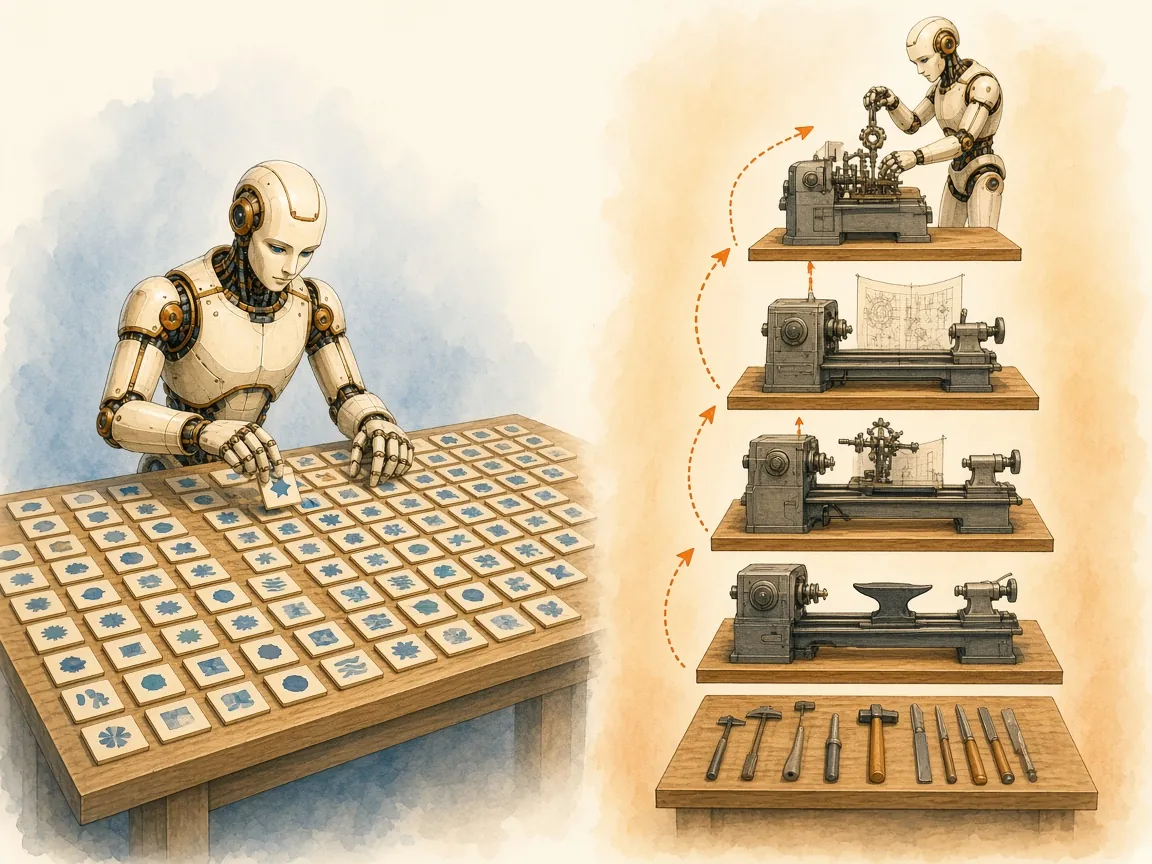
Transfer is the case in which learning a useful abstraction \(f_1\) lowers the cost of many later tasks, \(C(\text{task} \mid f_1) < C(\text{task})\). Recursive improvement requires \(f_1\) to lower the cost of discovering another abstraction \(f_2\),
\[C_{\text{discover}}(f_2 \mid f_1) < C_{\text{discover}}(f_2) ,\]
where \(f_2\) in turn lowers the cost of discovering \(f_3\), and so on. Recursive abstraction structure consists of chains \(f_1 \to f_2 \to f_3 \to \cdots\) in which each abstraction changes the search space for the abstractions after it.
A domain can be infinitely large and still lack such chains. Learning another word of a language helps a speaker use the language and leaves the cost of learning the next word about the same. The infinitely many arithmetic expressions that can be built from a fixed set of operators have unbounded size and bounded abstraction depth. Mathematics and software contain long chains. A lemma becomes a step in the proof of a stronger theorem, the theorem defines objects needed to state a new theory, and the theory compresses whole families of later arguments. A function becomes part of a library, libraries support frameworks, frameworks support domain-specific languages, and those languages support systems that generate programs. In both cases the results of earlier work become operations used in later work.
Discovery cost and time-bounded complexity
Kolmogorov complexity measures the length of a description and ignores the cost of finding it. If \(x_n\) is the \(n\)th object in a computable enumeration, such as the \(n\)th theorem of a formal system, a short program can run the enumerator until \(x_n\) appears. Then \(K(x_n \mid n) = O(1)\), even if finding \(x_n\) takes an astronomical amount of computation. Levin complexity adds the logarithm of running time to program length,
\[\mathit{Kt}_B(x) = \min_{p \,:\, U_B(p) = x} \bigl[\, |p| + \log_2 T(p) \,\bigr] ,\]
where \(B\) is the basis of primitives available to the universal machine \(U_B\), \(|p|\) is the length of program \(p\) in bits, and \(T(p)\) is its running time. Levin search, which runs every program with a share of time that decreases exponentially with its length, finds \(x\) in time on the order of \(2^{\mathit{Kt}(x)}\) (Gagliolo, 2007).
Let \(B_0 \subset B_1 \subset B_2 \subset \cdots\) be a growing library of persistent abstractions. The basis leverage of a later abstraction \(f_n\) is the reduction in time-bounded complexity that the accumulated library provides,
\[\Delta_n = \mathit{Kt}_{B_0}(f_n) - \mathit{Kt}_{B_{n-1}}(f_n) .\]
If search cost scales as \(2^{\mathit{Kt}}\), a frozen system searching from \(B_0\) and a recursive system searching from \(B_{n-1}\) have costs in the ratio
\[\frac{C_R(n)}{C_F(n)} \approx 2^{-\Delta_n} ,\]
so an unbounded additive advantage in description, \(\Delta_n \to \infty\), becomes an unbounded multiplicative advantage in search cost. Abstraction has large effects in this model because universal search prices description length exponentially.
A historical chain of dependencies can differ from a computational one. Mathematics may have developed \(f_1\), \(f_2\), and \(f_3\) in that order while a short direct proof of \(f_3\) from first principles exists, and in that case the apparent hierarchy provides little basis leverage. A claim of sustained RSI therefore needs a hardness condition, under which every program for \(f_n\) over the original basis is long or slow, so that \(\mathit{Kt}_{B_0}(f_n)\) stays large.
A sufficient condition follows from a model of the abstractions as nodes in a growing dependency graph. Suppose that every program that produces \(f_n\) from the original basis has to reconstruct its ancestors, at a cost of about \(W_n\) steps, so that \(\mathit{Kt}_{B_0}(f_n) \ge \log_2 W_n\). Suppose also that, with the accumulated library, \(f_n\) can be produced by \(a_n\) steps of new work and a program of \(s_n\) bits that selects the relevant ancestors and specifies the new step, so that \(\mathit{Kt}_{B_{n-1}}(f_n) \le \log_2 a_n + s_n\). Then
\[\Delta_n \ge \log_2 W_n - \log_2 a_n - s_n ,\]
and \(\Delta_n \to \infty\) whenever
\[\frac{W_n}{a_n\, 2^{s_n}} \to \infty .\]
The computation needed to rebuild the stack of abstractions from primitives has to grow faster than the cost of extending the stack by one step, including the cost of selecting what to reuse. The total object becomes harder to construct from scratch while each extension stays small, as in cumulative mathematics, where a proof that builds on a large body of earlier results is short compared with a proof from axioms. Under this condition the cost of each new step can stay manageable for the recursive system while the absolute difficulty of the problems grows to infinity.
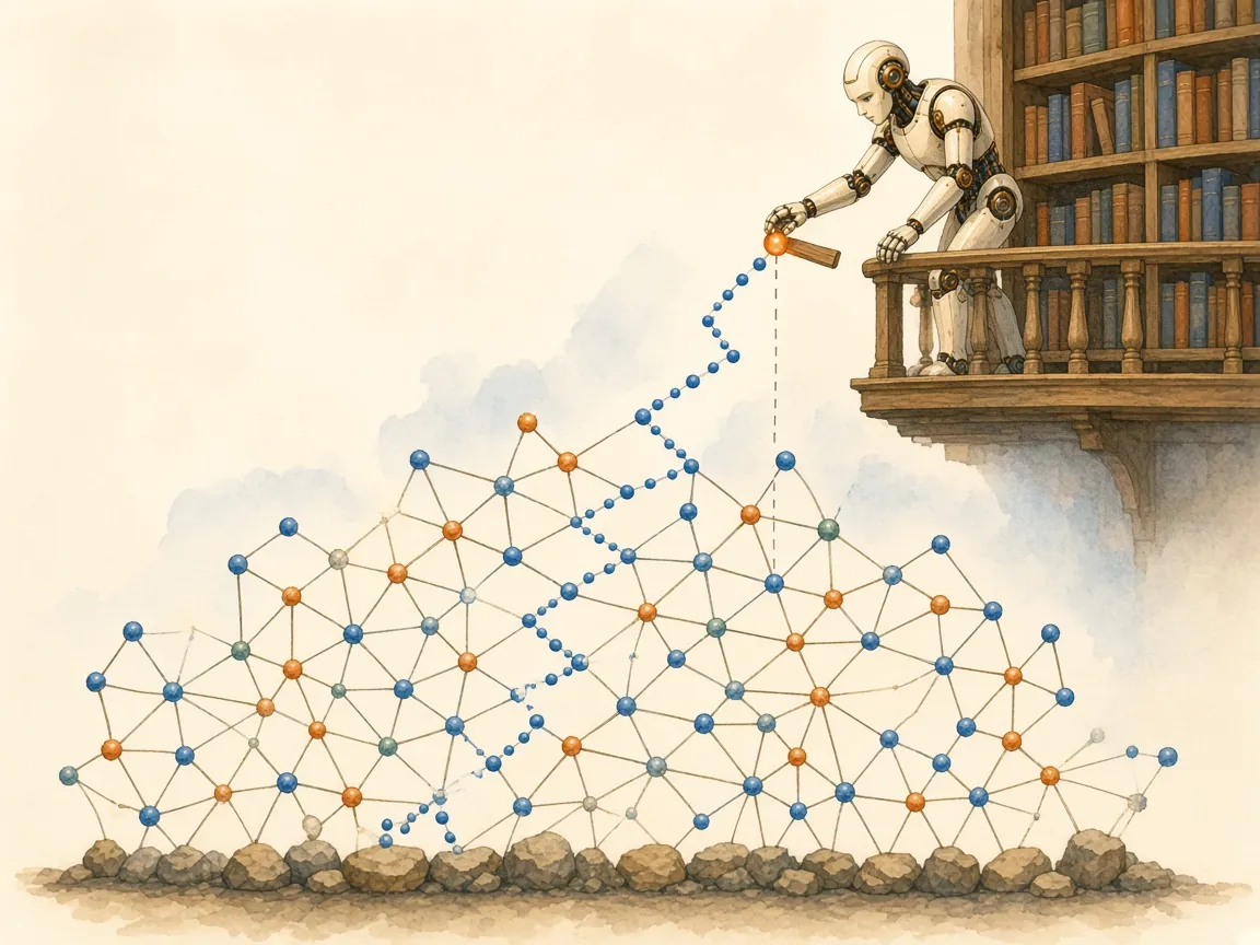
Random task streams
At the opposite extreme is an infinite binary task stream \(x = x_1 x_2 \ldots\) generated by fair coin flips. With probability one the stream is Martin-Löf random, and by the Levin–Schnorr theorem (Schnorr, 1973; Chaitin, 1975) its prefixes are incompressible up to a constant,
\[K(x_{1:n}) \ge n - O(1) ,\]
where \(K\) is prefix-free Kolmogorov complexity. Suppose a computable learner has accumulated reusable structure worth \(A_n\) bits, in the sense that its persistent representation together with a residual code describes \(x_{1:n}\) in \(n - A_n + O(1)\) bits. Then \(K(x_{1:n}) \le n - A_n + O(1)\), and the two bounds together give \(A_n = O(1)\). For almost every stream, the reusable compression accumulated by any computable learner stays bounded.
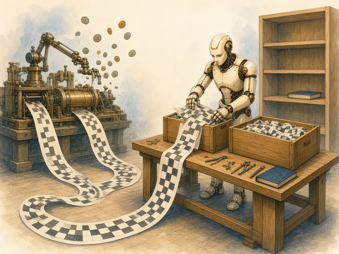
Applying the theorem to RSI takes one modeling assumption, that sustained RSI requires an unbounded reusable structural advantage. Under that assumption, RSI is impossible on generic random task streams. The phrase “almost every” refers to the fair-coin measure on infinite bit strings, and mathematics, code, language, and scientific data occupy small, highly structured subsets of all strings, so the result leaves real-world domains open. Together with the modeling assumption, the theorem shows that unbounded recursive leverage is a special property of a task stream and requires structure in the task generator.
Closed and open task generators
A second property of a task generator is where its new information comes from. A process \(X\) is algorithmically closed if a finite description \(\phi\) determines it, in the sense that \(K(X_{1:n} \mid \phi, n) = O(1)\) for all \(n\). The digits of \(\pi\), a deterministic Turing machine on a fixed input, a cellular automaton with fixed rules and initial state, and the enumeration of the theorems of a formal system are all closed. Their apparent complexity can grow forever while all of their algorithmic information stays in the finite description.
An open process keeps receiving new information. The cumulative exogenous information
\[E(n) = K(X_{1:n} \mid \phi, n)\]
stays bounded for a closed process. It is unbounded and sublinear, \(E(n) = o(n)\), for a sparsely open process, and it grows linearly, \(E(n) = \Omega(n)\), for a process with a persistent rate of innovation. Independent external information can be learned only after it arrives.
Closedness and recursive structure vary separately. A periodic sequence is closed and lacks chains of abstraction, while empirical physics is open, since new measurements keep arriving, and its theory may still admit long chains of abstraction. External information places a floor under the frontier difficulty \(H(\theta)\) and leaves the reusable leverage \(R(\theta)\) free to grow.
The same reasoning applies to data produced by people. Humans write mathematics, proofs, and code with a great deal of recursive structure, so human involvement is compatible with RSI. The quantity to track is the conditional novelty that remains after everything reusable has been learned. If progress in a domain keeps requiring human judgments, observations, experiments, or preferences that are independent of what is already known, those inputs contribute a part of the frontier difficulty that persists after every reusable regularity has been learned.

Finite persistent state
A separate limit comes from the learner. If every persistent part of a learner fits in \(M\) bits, the learner has at most \(2^M\) persistent states. If capability under a fixed evaluation protocol is a function \(Q\) of the persistent state, a sequence of strict improvements visits each state at most once and so contains at most \(2^M - 1\) improvements. An endless sequence of strict improvements therefore requires a persistent resource that grows, such as memory, model capacity, external storage, or an environment that serves as memory, and compression can only postpone the limit.
The bound is loose in practice. A system with enough state could go through a very long phase of recursive improvement before reaching it, and a finite ceiling can lie far above any current system.
Classification of domains
Recursive abstraction structure and the rate of new external information give a rough classification of domains. Formal mathematics and theorem proving have long chains of abstraction, since lemmas, theories, and proof methods become inputs to later discovery, and formal problems are almost entirely closed. Code and program synthesis have similar chains, from functions to libraries, domain-specific languages, compilers, and program generators, and need little new information when the specification is fixed and more when the requirements come from the world. The design of algorithms, optimizers, and machine-learning pipelines is recursive by construction, because improvements change the search that produces later improvements, and synthetic versions of these problems need little new information. Formal mathematics, code, and algorithm design are the strongest candidates for a high ceiling on recursive improvement, although unbounded improvement remains unproven for all three.
Circuit and hardware design have strong hierarchical reuse and automation, and physical constraints are likely to impose limits after a recursive phase. Closed games such as chess and Go have deep abstractions and search heuristics and receive zero new information, and their finite state spaces imply eventual saturation. Theoretical science combines long chains of abstraction with experiments that bring in new information, so recursive improvement of theory can proceed above an empirical floor. Natural language and literature have a great deal of hierarchy and transfer, while new meanings, culture, and preferences keep entering, and the case for unbounded recursion in them is weak. Medicine, social systems, and open-world prediction have large reusable latent structure and a persistent flow of new empirical information, which sets substantial floors. Random labels and random bits have zero reusable structure and the highest rate of new information, which rules out structural RSI.

Mathematics and code have several properties that favor RSI, although the unbounded case is open in both. They are compositional, their abstractions can operate on other abstractions, much of each problem can be made algorithmically closed, and outputs can often be checked cheaply. Cheap verification makes scalable training signals possible, and it enters the condition \(r > h\) only through its effect on the growth rates of reusable leverage and frontier difficulty.
Limits of the argument for mathematics
Recursive improvement in mathematics can saturate even though mathematical abstraction can be arbitrarily deep. Some families of theorems may have proof complexity that grows faster than any useful abstraction can offset. New theories may make some problems exponentially easier and leave others unchanged. A growing library increases the branching and selection costs of search, and the cost of finding and validating new abstractions may eventually exceed the savings they bring. Conceptual hierarchies that seem necessary can also be bypassed by different proofs.
In the other direction, Blum (1967) constructed computable functions for which every program has a faster program on all but finitely many inputs, so computation allows algorithmic improvement to continue forever. The functions come from diagonalization, and whether natural families of mathematical tasks behave the same way is an open empirical and theoretical question.
Transfer of learning efficiency across domains
The scalar model extends to a vector of capabilities \(\boldsymbol\theta = (\theta_{\text{math}}, \theta_{\text{code}}, \theta_{\text{language}}, \theta_{\text{science}}, \ldots)\) that evolves as \(d\boldsymbol\theta/d\log C = \boldsymbol\beta(\boldsymbol\theta)\). The matrix
\[\Gamma_{ij} = \frac{\partial \beta_i}{\partial \theta_j}\]
measures whether an improvement in capability \(j\) raises the rate at which capability \(i\) can be learned afterward. It gives a definite meaning to the question of whether reinforcement learning with verifiable rewards (RLVR) on mathematics and code produces something like the general factor \(g\) found in human test scores (Spearman, 1904). If training on mathematics raises \(\theta_{\text{math}}\) while \(\Gamma_{\text{language},\text{math}} \approx \Gamma_{\text{science},\text{math}} \approx 0\), the model has become better at mathematics and learns at the same rate elsewhere, and the frontier has moved along one axis. If \(\Gamma_{i,\text{math}} > 0\) across many unrelated held-out domains, training on mathematics has improved general learning efficiency, which is closer to a general factor.
An eigenvector of \(\Gamma\) with a positive eigenvalue is a combination of capabilities that raises its own rate of growth, which gives a local model of recursive amplification. A positive eigenvalue is weaker than unbounded takeoff, since \(\Gamma\) can change sign, resource limits can bind, and the eigenvalue can decay toward zero. The entries of \(\Gamma\) can be estimated by experiment.
Measuring a change in learning efficiency
The test is whether RLVR on mathematics and code makes new abilities in other domains cheaper to acquire. Higher scores on benchmarks outside mathematics and code could come from ordinary transfer of representations, so the protocol measures the compute needed to learn in each new domain, in five steps.
Save a sequence of checkpoints before and during a run of RLVR on mathematics and code, with the architecture and persistent resources held fixed.
Build held-out task generators in several unrelated domains, and supply the same amount of new human information at every checkpoint.
Calibrate a latent capability \(\theta_j\) for each domain with an item-level difficulty model, so that the density of task difficulty stays separate from the rate of learning.
Starting separately from each checkpoint, measure the compute needed to gain a fixed increment \(\Delta\theta_j\) in each new domain, which estimates \(\beta_j = \Delta\theta_j / \Delta\log C\).
Compare each checkpoint with a frozen-mechanism counterfactual. If later checkpoints need less compute to learn new abstractions outside mathematics and code, after controlling for installed facts, leakage between training and test tasks, and additional human data, training on mathematics and code has changed the improvement mechanism itself, beyond adding domain skill.

The protocol estimates the change \(\Delta\beta_j\) in the rate of learning. A gain \(\Delta\theta_j > 0\) in capability can come from transfer alone, while \(\Delta\beta_j > 0\) means the system improves faster in the domain, as recursive self-improvement requires.
Summary
The capability curve of an ideal learner depends on the structure of the tasks being generated. If the reusable structure in a domain is finite, the learner eventually extracts it and transfer saturates. If reusable structure grows about as fast as frontier difficulty, learning efficiency stays roughly constant and capability grows with log compute. If earlier abstractions keep becoming tools for discovering later ones, reusable leverage can grow faster than frontier difficulty, and the scaling law itself improves. The three cases correspond to \(r < h\), \(r = h\), and \(r > h\).
Mathematics and code are plausible candidates for the third regime because they appear to contain long chains in which each abstraction becomes part of a better language for searching for the next one. Many other domains contain a large amount of transferable structure with weak evidence of such chains. In those domains, learned abstractions make applications cheaper while the cost of discovering new abstractions stays about the same.
Identifying RSI in a system requires comparing an evolving improvement mechanism with a frozen counterfactual under matched resources. Whether RSI can be sustained depends on the structure of the tasks. A learner can build only on structure that the task-generating process contains, and sustained RSI requires a process in which learned representations repeatedly lower the cost of discovering more powerful ones. Infinite task sets, compositionality, transfer, and cheap verification are each weaker conditions. Whether a capability curve flattens, follows its scaling law, or accelerates depends on how fast reusable leverage grows relative to frontier difficulty, and both rates depend on the domain as well as on the model.